Deep neural networks excel in many difficult tasks, given large amounts of training data and enough processing power. The neural network architecture is an important factor in achieving a highly accurate model, and normally state-of-the-art results are obtained by building up on many years of effort, by hundreds of researchers (see examples in Szegedy et al., 2015, (He et al., 2016)[https://arxiv.org/abs/1512.03385] for more details). Techniques to automatically discover these neural network architectures are, therefore, very much desirable. As part of the AutoML project at Google, this paper was published in ICML 2017 (Real et al., 2017), with the aim of discovering deep neural network (DNN) architectures without any human participation. The proposed method is simple and is able to generate a fully trained network requiring no post-processing. While previous work in Morse et al. 2016, He et al. 2016 focused on small neural networks, these small networks are not scalable, as it’s deep neural networks that are needed for achieving state-of-the-art in image classification.
Overall approach
The heart of the proposed method is an evolutionary algorithm (EA). An EA is a population-based optimization algorithm that, inspired by biological evolution, evolves a population of candidate individuals, by repeatedly performing operations such as reproduction, mutation, recombination (crossing-over), and selection. A fitness function determines the quality of each individual. The authors employ a modified version of the EA, described above such that a population of simple neural network architectures and their hyper-parameters are evolved while the weights are adjusted using back propagation.
Initial conditions
Each evolutionary experiment begins with a population of simple models, consisting of a single-layer with no convolutions and a learning rate of 0.1. This poor initial condition forces evolution to make the discoveries itself, rather than allowing the experimenter to “rig” the experiment by hand picking initial conditions.
Evolution process
Next, the models are evolved, using only mutation operations. The authors define a set of 11 types of mutation operations, all of which are designed to be very similar to what a human network designer does to improve an architecture.
The operators include: altering the learning rate, “identity” (keep training), weight reset, insert/remove convolutions, add/remove skip connections, insert a one-to-one/identity connection, and alterations of stride size, number of channels, and filter size.
While the authors explored the use of several recombination operations, they found that these recombinations did not improve their results. The fitness of each individual is calculated as the accuracy of the discovered neural network on a validation set.
Each individual architecture plus a learning rate form the individual’s DNA, which is implemented in TensorFlow. The vertices in this graph represent activations, such as ReLU and Linear functions. The edges represent either an identity function or a convolution layer containing mutable numerical parameters which define the convolution operation. During evolution, when multiple edges are incident on a vertex, they each must be of the same size and have the same number of channels for their activations. If not, this inconsistency is resolved by choosing one incoming edge to be the primary input, reshaping the rest using zeroth-order interpolation for the size, and truncating/padding for the number of channels. Mutation on a numerical parameter chooses the new value at random around the existing value. This makes it possible for the evolutionary process to choose any number within this range that gives better accuracy.
At each step of the evolutionary process, two individuals are randomly selected from the population by a computer, referred to as a worker. The individual with lower fitness is killed right away. A new child (a new DNN architecture) is created by applying a mutation operation (randomly selected from the predefined set of mutations) to the surviving individual. The child is trained, its fitness value is computed, and becomes “alive” as it’s added back to the population. If a child’s layer has matching shapes with that of its parent, the weights are preserved. This helps to retain some of the learned weights during the evolutionary process instead of learning them from the scratch. This process is repeated for a long time (about 12 days based on the experiments).
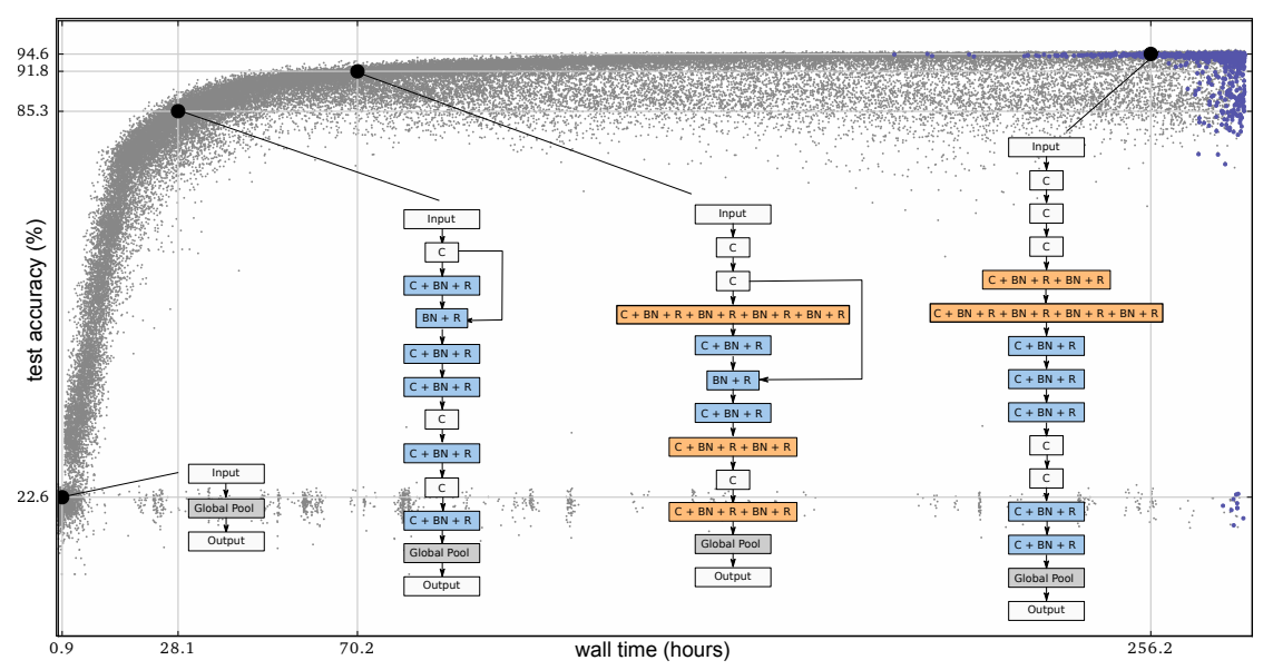 Figure 1 Progress of an evolution experiment. Each dot represents an individual in the population. Blue dots (darker, top-right) are alive. C: convolution, BN: batch normalization, R: Relu
Training and validation
For DNN training, the authors used SGD with momentum of 0.9, a batch size of 50, and a weight decay of 0.0001 for regularization. Cross-entropy is used as the loss function. Each training runs for 25,600 steps. For both CIFAR-10 and CIFAR-100, the training set consists of 45000 samples, with 5000 samples held out for validation. The training set is augmented as in He et al. 2016.
The authors employed a massively-parallel, lock-free infrastructure of 250 workers, and many of them operate asynchronously on different computers with no direct communications. The whole population, consisting of 1000 individuals, is stored in a shared file-system that all the workers have access to.
Experimental results
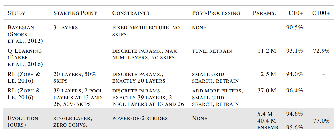
To test the proposed method, CIFAR-10 and CIFAR-100 were selected as these two datasets require large neural networks to obtain good results. Due to result variability, the experiments were repeated five times and the top models obtained a test accuracy of 94.6% for CIFAR-10 and 77% for CIFAR-100. The authors claim that these are the most accurate results obtained for these datasets by using automated discovery methods that start from trivial initial conditions. However, the obtained results are a little worse than the results in Wide ResNet (Zagoruyko and Komadakis, 2016) and DenseNet (Huang et al., 2016) that obtained (96.2%, 81.7%) and (96.7%, 82.8%) on (CIFAR-10, CIFAR-100) respectively.
Effect of population size and number of training steps:
Increasing both population size as well as the number of training steps broaden the model search space; as a result, it improves the test accuracy until reaching a plateau.
Conclusion
This paper shows that EA is able to fully automate the discovery of deep neural net architectures that are capable of solving complex tasks. Although the authors claim that their method is scalable, its use requires a large-scale infrastructure. The authors hope that future algorithmic and hardware improvements will allow implementation to be more economical. Overall, the proposed method is a promising approach for automating scalable architectural design of DNNs.